On the same pipeline, the synthetic stand-in scored a third higher than the real corpus.
The stand-in erased the participant correlation, so a leakage audit run on synthetic data passes whether or not the real data leaks.
A synthetic stand-in is usually validated by showing that its descriptive statistics match the source.
In 2025 I could not open the COLET corpus, so my paper said the stand-in preserved those statistics, and nobody, including me, could compare the two. Privacy rules and scarce recordings put many studies in the same spot. Once the corpus was open, I compared them.
So I wrote the decoder
In 2025 I built the proof of concept, a classifier trained on a synthetic stand-in because the corpus ships as MATLAB v7.3 tables that no standard Python reader could decode. This year I wrote the decoder (mat73-reader, on PyPI) and opened the real recordings. Then I ran that pipeline, unchanged, on the stand-in and on the real corpus, with ungrouped and with participant-grouped 5-fold cross-validation. That is the 2×2 on the result slide.
47 participants in four visual-search conditions, 188 labeled task instances.
Each task ended with a raw NASA-TLX[2] (RTLX, the unweighted mean of six subscales), and my primary label is the top tertile of that mean. The 2×2 keeps the proof of concept's ten features: gaze dispersion, pupil diameter[4, 5], gaze velocity, and the fixation and saccade rates. The honest protocol adds two blink features, twelve in all, z-scored within each participant.
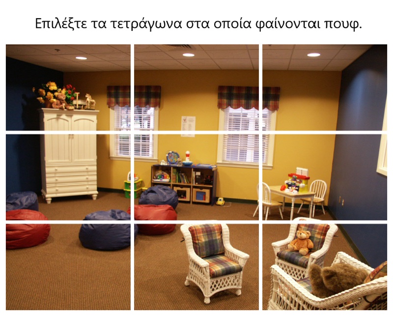
COLET[1], Ktistakis et al. 2022. One of its 21 search screens, as a participant saw it: “Select the squares in which pouffes are visible.” Five screens per condition, one rating after each block of five.
The COLET experiment →Screens: COLET, Ktistakis et al. 2022, Computer Methods and Programs in Biomedicine; Zenodo 7766785, CC BY 4.0. Photographs: Quattoni and Torralba 2009, MIT Indoor Scenes. The COLET authors added the grid and the instructions.
On the same pipeline, the synthetic stand-in scored a third higher than the real corpus.
Amber is the synthetic stand-in, blue the real corpus with the tertile label.
Every cell is macro F1, mean (SD) across five folds, on the same pipeline and features. The proof of concept replicated exactly on its own split first: positive-class F1 0.897, macro 0.916.
Where the 0.897 came from
0.916macro F1, synthetic stand-inThe proof of concept on its own split: macro F1 0.916. The dashed line is the reported 0.897, the same split in positive-class F1.
The two metrics differ by 0.02 to 0.15 across these cells. The axis starts at 0.5.
Participant 5, thirty seconds in each task
Thirty seconds of participant 5's gaze in each task, with nothing simulated. Dot size is pupil diameter at the last sample. Colors match the poster panel.
The stand-in, measured
The 2025 generator drew every feature and subscale from one hand-set difficulty term, with no participant term and no corpus statistic behind it. A stand-in fitted to the real means, SDs and correlations scored 0.555 (0.048, 25 draws), below the corpus's 0.623 on the same pipeline, so the moments carry none of the inflation.
Each block is one participant, one eye per condition: search only, then with time pressure, then counting, then both. Pupil size is that block's mean pupil diameter, from the corpus and from the archived 2025 stand-in, sorted by each person's average.
The model, running right here
The 2×2 kept the 2025 pipeline as it was. Here I z-scored each feature within the participant, added two blink features, ran five participant-grouped folds over five seeds, and reported macro F1 with its SD. A twelve-coefficient logistic regression matched or beat three tree ensembles. It runs in this page.
Probability of high load from the frozen winner's twelve coefficients, fitted on all 188 rows for this demo; 0.783 is its cross-validated score. Sliders are standard deviations from your own calm baseline; the two profiles are the corpus's class means. Arrow keys move a focused slider; Escape releases it. The gauge's pupil follows the mean pupil slider.
Six subscales, one negative control
Mental demand scores highest, with effort within one SD of it. Physical demand sits at chance, as a model of cognitive load[3] should.
The label sweep
The score moves with where TLX is cut into high and low, so I fixed the top tertile before running the sweep.
Top tertile, primary: the positive class is 36% of instances. Same model, same twelve features, same 25 participant-grouped folds. Only the labeling changes.
The same audit, pointed at my own decoder
The accepted abstract reports 0.762. My decoder, mat73-reader, turned every empty blink table into two phantom rows and contaminated the blink features in 40 of 188 instances. An independent decoder disagreed on those tables and no others. I fixed the decoder and rebuilt the features with the protocol unchanged. Every cell without blink features reproduced, and 0.762 became 0.783. The audit of the stand-in needed the same audit on my own decoder.
Each square is one labeled instance, grouped by participant as on the measured slide. The 40 lit squares are the instances whose blink tables were empty, read from the contaminated and the corrected feature files.
What I found
- 1
Most of the inflation was structure the generator fabricated, some was the luck of one split, and almost none was leakage.
- 2
The checks that caught it are standard and need no new data: grouped validation, a label sweep, and a negative control, all run on the real data.[6, 7]
- 3
With one corpus and one generator, n = 188, I have shown that this can happen and have not measured how often it does.
What a Synthetic Stand-In Hid: Decomposing an Inflated Eye-Tracking Benchmark of Cognitive Load. William Garrow, Boston University, Boston, MA · Georgia Institute of Technology, Atlanta, GA. Thanks to the COLET authors for releasing the corpus.